In the first part of this tutorial, I covered the basics of image processing - viewing images as data, iterating through pixels, and performing basic operations. This part will cover the idea of image convolution, and future parts will go on to discuss some of the more popular uses of the technique.
As the field of image processing is heavily influenced by mathematicians, there are reams of unnecessarily complex equations surrounding image convolution. I don’t like that. In this tutorial, I will explain the concepts, show you some logic, and then tack on the equations at the end.
Additionally, I want to move away from working with images directly. Remember from the first part that image pixels are stored as ints. As we get into increasingly complex filters, the rounding error associated with operating directly on ints will get annoying. Let’s avoid this by approaching image processing in the following manner:
This will slow down our code slightly, but it will save us from having to deal with rounding error and pixel location logic.
The code to do steps 1 and 3 is simple enough. For a black-and-white image, we just need to iterate.
/**
 * Converts black-and-white PImage to float[][]
 */
float[][] toArray(PImage img) {
  float[][] values = new float[img.width][img.height];
  img.loadPixels();
  for(int x = 0; x < img.width; x++) {
    for(int y = 0; y < img.height; y++) {
      values[x][y] = brightness(img.pixels[x + y * img.width]);
    }
  }
  return values;
}

/**
 * Converts a float[][] to a normalized black-and-white PImage
 */
PImage toImage(float[][] values) {

  // Scale values to [0, 255]
  float maximum = 0, minimum = Float.MAX_VALUE;
  for(int x=0; x<values.length; x++) {
    for(int y=0; y<values[0].length; y++) {
      maximum = max(maximum, values[x][y]);
      minimum = min(minimum, values[x][y]);
    }
  }
  for(int x=0; x<values.length; x++) {
    for(int y=0; y<values[0].length; y++) {
      values[x][y] = (values[x][y]-minimum)/(maximum-minimum) * 255.0;
    }
  }

  PImage img = createImage(values.length, values[0].length, ALPHA);
  img.loadPixels();
  for(int x = 0; x < img.width; x++) {
    for(int y = 0; y < img.height; y++) {
      img.pixels[x + y * img.width] = color(int(values[x][y]));
    }
  }
  img.updatePixels();
  return img;
}
If you want to generalize this to colors, you can substitute a [ red, green, blue ]
array for each element (so you’d have a float[][][]). For now, I’m sticking
with black-and-white images. Color images would obfuscate the core concepts of
the tutorial.
Let’s start talking about convolution. In the first section, we iterated through pixels one at a time. Writing loops like
for(int x=0; x<img.width; x++) {
  for(int y=0; y<img.height; y++) {
    // Do stuff
  }
}
produced the following iteration pattern

All the logic we could create came from information about these solitary pixels. However, most interesting information comes from groups of pixels. Most likely, we care about a pixel’s neighbors. What color are they? Are there any noticeable patterns? This is the issue that image convolution addresses. Rather than iterating through every pixel linearly, we will iterate around each pixel’s neighbors. For example, if we were only concerned with a pixel’s immediate neighbors, our new iteration scheme would look like
for(int x=0; x<img.width; x++) {
  for(int y=0; y<img.height; y++) {
    // Current center pixel is at (x, y)
    for(int u=-1; u<=1; u++) {
      for(int v=-1; v<=1; v++) {
        // Current neighbor is at (x+u, y+v)
      }
    }
  }
}
and would produce a pattern like
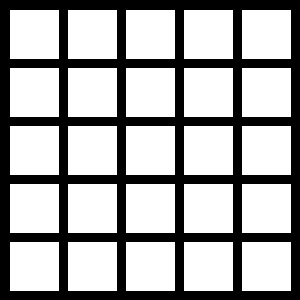
Here, the blue square represents the center pixel, and iterates in the same pattern as before. The green square is the current pixel that the code’s inner loop is evaluating. Take some time to understand how the above code translates into the shown iteration scheme.
Now, what do we do with all this extra iteration? In convolution, we take a weighted average of all the neighbor pixels and use it to update the center pixel of an output image. In the simplest example, let’s weight all the neighbors equally. Our weights look like
\( \left[\begin{array}{ccc} 1/9 & 1/9 & 1/9 \\ 1/9 & 1/9 & 1/9 \\ 1/9 & 1/9 & 1/9 \end{array}\right]\)
In Processing, this operation looks like
/**
 * Convolves a float[][] representation of an image with a kernel of weights
 */
float[][] convolve(float[][] img, float[][] kernel) {
  int xn, yn;
  float average;

  // Showcasing how to access width and height of nested array
  int w = img.length;
  int h = img[0].length;
  float[][] output = new float[w][h];

  // Iterate through image pixels
  for(int x=0; x<w; x++) {
    for(int y=0; y<h; y++) {

      // Iterate through kernel values to get weighted average
      average = 0;
      for(int u=0; u<kernel.length; u++) {
        for(int v=0; v<kernel[0].length; v++) {

          // Get associated neighbor pixel coordinates
          xn = x + u - kernel.length/2;
          yn = y + v - kernel[0].length/2;

          // Make sure we don't go off of an edge of the image
          xn = constrain(xn, 0, w-1);
          yn = constrain(yn, 0, h-1);

          // Add weighted neighbor to average
          average += img[xn][yn] * kernel[u][v];
        }
      }
      // Set output pixel to weighted average value
      output[x][y] = average;
    }
  }
  return output;
}
and, when run on this picture of my living room, produces
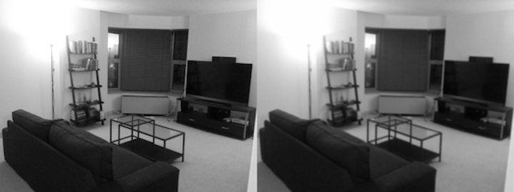
Hmm, that ever so slightly blurred the image. If you think about what we just did, that makes sense. Every pixel’s value was influenced by its neighbors, so local jumps in pixel brightness were tapered.
I promised you some mathematics, so here it is.
\((f*g)(x,y) = \iint f(x-u,y-v)g(u,v)\,du\,dv\)
I wrote the equation applied to the “special” case of images, although, in image processing literature, you usually see the generalized n-dimensional vector version. Just in case you come across an n-dimensional image. Or something.
I used \(x\), \(y\), \(u\), and \(v\) to coincide with the variables in the above code.
\(f\) is the image, and \(g\) is the matrix of weights. Remember that an integral
operator applied to discrete information is just a sum, and you can see how the
entire equation is nothing more than a weighted average.
One nice thing about the math is the introduction of an asterisk as shorthand
for convolution, \(f*g\). You’ll see this operator in a lot in image-processing
papers, so keep it in mind if you’re reading up on the topic.
So, what can we do with convolution? The set of weights we choose - or the kernel - can create a wide range of outputs. In the next few sections, we will explore some of the most common kernels. The next section will cover one of the most useful data mining skills - estimating gradients.