In the previous section, we discussed the idea of image convolution, which allows us to gather information on groups of pixels. What can we do with this? Well, a lot. Let’s start simple.
Remembering that images are data, we can start thinking about slopes. The data
has two dimensions, \(x\) and \(y\), so it has two gradients,
\(\Delta f / \Delta x\) and \(\Delta f / \Delta y\). Seeing how
\(\Delta f\) is just \(f_2 - f_1\), you could design a 3x3 kernel to get
your slopes like so:
\(
g_x = \left( \begin{array}{ccc}
0 & 0 & 0\\
0 & -1 & 1\\
0 & 0 & 0
\end{array} \right)\qquad
g_y = \left( \begin{array}{ccc}
0 & 0 & 0\\
0 & -1 & 0\\
0 & 1 & 0
\end{array} \right)
\)
Here, we’re ignoring most of the neighbors by setting their weights to zero. The remaining weights simplify out to a difference of pixels. This is functional, but as I said in Part 1, images are a lot of data. We have pixels to spare. Enter the Sobel operator, which extends the above definition to use more of the neighbor pixels.
\(
g_x = \left( \begin{array}{ccc}
-1 & 0 & 1\\
-2 & 0 & 2\\
-1 & 0 & 1
\end{array} \right)\qquad
g_y = \left( \begin{array}{ccc}
-1 & -2 & -1\\
0 & 0 & 0\\
1 & 2 & 1
\end{array} \right)
\)
The idea is the same here, but now the slope estimates are a little more resistant to noisy data messing things up.
Not to be outdone (or not to miss out on easy publications), others have jumped
on the make-up-a-gradient-kernel bandwagon. Chief among these is the Scharr operator,
which purports to be a better approximation of derivatives that don’t fall nicely
on the \(x\) or \(y\) axis.
\(
g_x = \left( \begin{array}{ccc}
-3 & 0 & 3\\
-10 & 0 & 10\\
-3 & 0 & 3
\end{array} \right)\qquad
g_y = \left( \begin{array}{ccc}
-3 & -10 & -3\\
0 & 0 & 0\\
3 & 10 & 3
\end{array} \right)
\)
We can convert the \(x\) and \(y\) derivative approximations to polar
coordinates with \(r = \sqrt{x^2 + y^2}\) and \(\theta = \arctan{y / x}\).
By representing \(\theta\) as color, the magnitude-and-direction view of 2D
gradients allows us to show the output of gradient convolution on a single image.
It would be messy to edit our old toImage function to do this, so let’s make a
new showDerivative method.
/**
 * Creates an image showing gradient as mag, direction
 */
PImage showDerivative(float[][] img, String type) {
   float[][] dx, dy, magnitude, direction;
   float maximum, minimum;
   int luminosity;
   color col;

   // Get directional derivatives
   if(type.equals("Scharr")) {
     dx = scharrXGradient(img);
     dy = scharrYGradient(img);
   }
   else if(type.equals("Sobel")) {
     dx = sobelXGradient(img);
     dy = sobelYGradient(img);
   }
   else {
     dx = xGradient(img);
     dy = yGradient(img);
   }
   // Convert to radial notation
   magnitude = new float[img.length][img[0].length];
   direction = new float[img.length][img[0].length];
   maximum = 0; minimum = Float.MAX_VALUE;
   for(int x=0; x<img.length; x++) {
     for(int y=0; y<img[0].length; y++) {
       magnitude[x][y] = sqrt(pow(dx[x][y], 2) + pow(dy[x][y], 2));
       maximum = max(maximum, magnitude[x][y]);
       minimum = min(minimum, magnitude[x][y]);
       // Direction is in the range [-pi/2, pi/2]
       direction[x][y] = atan(dy[x][y]/dx[x][y]);
     }
   }

   PImage output = createImage(img.length, img[0].length, RGB);
   output.loadPixels();
   for(int x=0; x<output.width; x++) {
     for(int y=0; y<output.height; y++) {
       luminosity = int(255.0 * (magnitude[x][y]-minimum) / (maximum-minimum));

       // Map gradient direction to one of four colors
       if(direction[x][y] >= -PI/2 && direction[x][y] < -PI/4)
         col = color(luminosity, 0, 0);
       else if(direction[x][y] >= -PI/4 && direction[x][y] < 0)
         col = color(0, luminosity, 0);
       else if(direction[x][y] >= 0 && direction[x][y] < PI/4)
         col = color(0, 0, luminosity);
       else
         col = color(luminosity, 0, luminosity);

       output.pixels[x + y * output.width] = col;
     }
   }
   output.updatePixels();
   return output;
}

/**
 * Estimates df/dx lazily
 */
float[][] xGradient(float[][] img) {
  float[][] gx = { { 0.0,  0.0, 0.0 },
                   { 0.0, -1.0, 1.0 },
                   { 0.0,  0.0, 0.0 } };
  return convolve(img, gx);
}

/**
 *  Estimates df/dy lazily
 */
float[][] yGradient(float[][] img) {
  float[][] gy = { { 0.0,  0.0, 0.0 },
                   { 0.0, -1.0, 0.0 },
                   { 0.0,  1.0, 0.0 } };
  return convolve(img, gy);
}

/**
 * Estimates df/dx using Sobel kernel
 */
float[][] sobelXGradient(float[][] img) {
  float[][] gx = { { -1.0, 0.0, 1.0 },
                   { -2.0, 0.0, 2.0 },
                   { -1.0, 0.0, 1.0 } };
  return convolve(img, gx);
}

/**
 *  Estimates df/dy using Sobel kernel
 */
float[][] sobelYGradient(float[][] img) {
  float[][] gy = { { -1.0, -2.0, -1.0 },
                   {  0.0,  0.0,  0.0 },
                   {  1.0,  2.0,  1.0 } };
  return convolve(img, gy);
}

/**
 * Estimates df/dx using Scharr kernel
 */
float[][] scharrXGradient(float[][] img) {
  float[][] gx = { { -3.0,  0.0, 3.0 },
                   { -10.0, 0.0, 10.0 },
                   { -3.0,  0.0, 3.0 } };
  return convolve(img, gx);
}

/**
 *  Estimates df/dy using Scharr kernel
 */
float[][] scharrYGradient(float[][] img) {
  float[][] gy = { { -3.0, -10.0, -3.0 },
                   {  0.0,   0.0,  0.0 },
                   {  3.0,  10.0,  3.0 } };
  return convolve(img, gy);
}
This function can be run with each of the three gradient-approximation kernels. Below is the unedited image (top left), and then the basic (top right), Sobel (bottom left), and Scharr (bottom right) kernels.
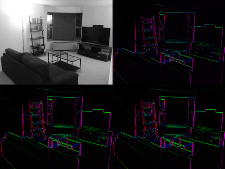
The basic gradient is the worst of the approximations, but the Sobel and Scharr aren’t all that different. For this reason, you’ll usually see the Sobel operator used in literature.
You can probably guess the mathematical representation of this stuff. You’ll
see the image represented as a two-parameter function \(f(x,y)\), or, more
pompously, the n-dimensional \(f(\textbf{x})\), where \(\textbf{x}\) is the
generalized vector including \(x\) and \(y\). The derivatives are then some
combination of \(\delta f / \delta x\), \(\delta f / \delta y\),
\(\delta f / \delta r\), \(\delta f / \delta \theta\), and
\(\delta f / \delta \textbf{x}\). Either way, a lot of partial derivatives.
Remember that it’s all just a bunch of people guessing at how to calculate
slopes, and you’ll be fine.
In the next section, we will generalize convolution to include larger groups of pixels and improve our smoothing function from Part 2.