The need to extract information from images and videos is a perennial issue in experimental work. As such, scientific image processing is a topic I’ve been wanting to address for some time now. This represents the first of a six-part tutorial focusing on what I consider to be the core of image processing. With the tools shown in these lessons, you will be able to automate the analysis and interpretation of experimental work, simultaneously decreasing human error and reducing the amount of time you have to spend in the lab.
In this post, I will go in to the fundamentals of image processing. This covers viewing images as data and creating basic logic to extract information from experimental images. Future posts will focus on the latter topic, extending into the field of computer vision and image processing algorithms.
All code examples are written in Processing, a really fun Java superlanguage focused on, well, processing images. If you’re at all interested in computer vision, I’d highly recommend looking into it. For those of you who don’t mind approaching image processing as a magical black box, Matlab has a solid toolkit, and, if you’re a little more code savvy, OpenCV is downright awesome. That being said, black box + science is always a terrible idea, and I claim no responsibility for misinterpreted data. Read the damn tutorial.
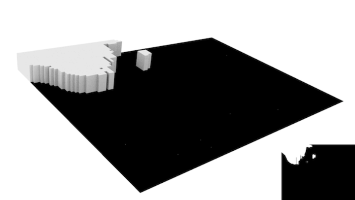
The 3D visualizations were done in Blender. The script I used to do so is stored in a Github repo here.
As a starting point, consider black-and-white images. These are very common in small-scale science, as color isn’t really a thing when you’re talking sizes smaller than visible light wavelengths (think SEM output and the like). So, as an example, here’s a grayscale image I took of my living room.
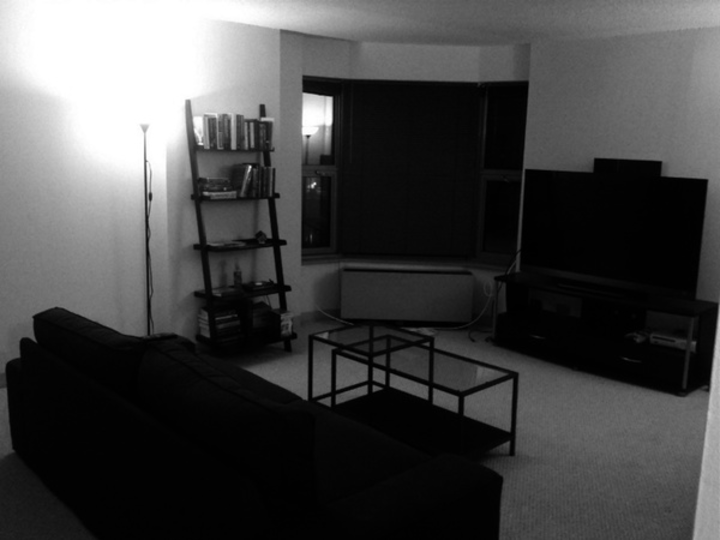
Digital images, not surprisingly, are composed of pixels. In the case of black-and-white images, each pixel can take an integer value from 0 to 255. 0 is black, 255 is white. The sample image is 800 x 600 pixels, so it consists of (800*600) 480,000 data points. Which brings me to my next point:
In the small sample image above, we’re dealing with half a million numbers. Full-res SEM images can be 5,000 x 5,000 pixels, representing 25 million data points. In many bio experiments, you have full-fledged videos of cells and whatnot. A 1080p RGB 30 fps video camera is producing (1920*1080*3*30) 186.6 million data points per second. That’s enough space to store the entirety of Moby Dick 200 times over!
Why am I emphasizing this so much? Simple: keeping this in mind will save you headaches (ie. crashed laptops) when we get to data manipulation. If you’re processing a lot of images, don’t be afraid of scaling down the size (in fact, this is a good approach to reduce noise!).
To convert the image above into a more mathematical notation, we are dealing with an 800 x 600 matrix of numbers. So, what can we do with this representation? The short answer: a lot. Let’s start with some simple ideas and get coding.
First, here’s a plot of a downsized version of the input image. Take this as our starting point - we’ll move forward from here.
Without any manipulation, you can already see some patterns. The furniture is dark, which means that the data in that area will have low values (remember that pure black is 0). Contrasting this is the light source in the top left, which is producing a region of pure white. The remaining data - the walls and floor - are slightly noisy gray areas. Let’s use this information to write our first image processing functions.
In Processing, we can iterate through the pixels of an image easily enough.
/**
 * Iterates through all of the pixels in an image
 */
PImage iterate(PImage img) {
  img.loadPixels();
  for(int x = 0; x < img.width; x++) {
    for(int y = 0; y < img.height; y++) {
      int loc = x + y * img.width;
      img.pixels[loc] = // Do something here!
    }
  }
  return img;
}
The only confusing aspect of this code is the loc = x + y * img.width line.
This is simply a conversion between our 2D representation of images and how the
pixels are actually stored in the computer. Not a big deal.
Using this, we can play around with some ideas. We know that the furniture is
black and the lights are white. Let’s use that to create functions findFurniture
and findLights. First, findFurniture:
/**
 * Highlights all dark pixels in an input image
 */
PImage findFurniture(PImage img) {
  PImage output = createImage(img.width, img.height, 'L');
  img.loadPixels();
  output.loadPixels();
  for(int x = 0; x < img.width; x++) {
    for(int y = 0; y < img.height; y++) {
      int loc = x + y * img.width;

      // If the input pixel is dark, highlight the output pixel
      int col;
      if(brightness(img.pixels[loc]) < 60) {
        col = 255;
      }
      // Otherwise, the output pixel is black
      else {
        col = 0;
      }
      output.pixels[loc] = color(col);
    }
  }
  output.updatePixels();
  return output;
}
This function iterates through the pixels of the living room image. If a pixel is dark (ie. if it’s furniture), then place a white pixel in the output image. Otherwise, place a black pixel. The output looks like this:
All in all, it did a decent job of finding the furniture in the image. We can use the same logic to find the lights, now looking for light areas instead of dark ones.
/**
 * Highlights all bright pixels in an input image
 */
PImage findLights(PImage img) {
  PImage output = createImage(img.width, img.height, 'L');
  img.loadPixels();
  output.loadPixels();
  for(int x = 0; x < img.width; x++) {
    for(int y = 0; y < img.height; y++) {
      int loc = x + y * img.width;

      // If the input pixel is light, highlight the output pixel
      int col;
      if(brightness(img.pixels[loc]) > 230) {
        col = 255;
      }
      // Otherwise, the output pixel is black
      else {
        col = 0;
      }
      output.pixels[loc] = color(col);
    }
  }
  output.updatePixels();
  return output;
}
Here, the light in the top left and its window reflection are highlighted.
This approach is aptly called threshold filtering, and it’s super easy. Believe it or not, it’s enough to solve a lot of image processing dilemmas in science. For example, let’s say we want to track the purple nucleus of a dyed cell. The function:
/**
 * Finds the nucleus of a cell using the fact it's purple
 */
PImage findNuclei(PImage img) {
  PImage output = createImage(img.width, img.height, 'L');
  img.loadPixels();
  output.loadPixels();
  for(int x = 0; x < img.width; x++) {
    for(int y = 0; y < img.height; y++) {
      int loc = x + y * img.width;

      // If the input pixel has red and blue elements, highlight it
      int col;
      if(blue(img.pixels[loc]) > 100 && red(img.pixels[loc]) > 50) {
        col = 255;
      }
      // Otherwise, the output pixel is black
      else {
        col = 0;
      }
      output.pixels[loc] = color(col);
    }
  }
  output.updatePixels();
  return output;
}
yields the output

One thing to note is that we’re now working with color images. This is very
similar to working with black-and-white images, but now we have even more data!
A color image generally breaks down into red, green, and blue channels,
which Processing allows you to access with red(), green(), and blue()
functions. Convenient, right? You can use differences in color as thresholds;
it’s the same thing we did before with brightness, but much more expressive.
Take some time to play around with these ideas. A lot of scientific image processing can be done with the techniques shown here mixed with a healthy dose of intuition.
In the next post, I’ll tackle image convolution. From there, we’ll discuss some of the most popular filters.