Okay, so we’ve worked with pixels and their immediate neighbors, but what about the non-immediate neighbors? Easily enough, we can include them by increasing our kernel size. The previous 3x3 kernels cover immediate neighbors, 5x5 kernels go two steps away, 7x7 is three steps, and so on. Cool, let’s do something with this.
What if, rather than weighting all neighbors equally, we weight them based off of their distance to the center pixel? Neighbors close to the center will have a greater weight, and more distant neighbors will be weighted less. We could make our own kernel and randomly fill in numbers that do this, but that wouldn’t allow mathematicians to write one of their favorite equations:
\(g(u,v) = \frac{1}{2\pi\sigma^2}e^{-\frac{u^2+v^2}{2\sigma^2}}\)
This is a two-dimensional version of the Gaussian function. Will it produce dramatically different results than randomly picking numbers? Nah, not really. But it’s a standard, so let’s use it.
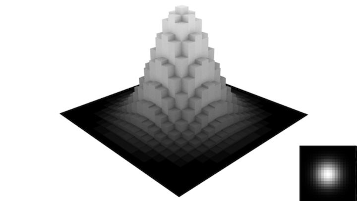
All that really matters here is the general shape. It peaks in the center and
decays as you move away. You can control how quickly it decays by varying the
\(\sigma\) parameter. Bigger sigma, slower decay. Let’s generate a 21x21 matrix of values from this function and use it as our kernel in convolution.
In our previous notation, this looks like a total mess:
\(
\begin{pmatrix}
7.93e-07 & 2.28e-06 & \cdots & 2.28e-06 & 7.93e-07 \\
2.28e-06 & 6.55e-06 & \cdots & 6.55e-06 & 2.28e-06 \\
\vdots & \vdots & \ddots & \vdots & \vdots \\
2.28e-06 & 6.55e-06 & \cdots & 6.55e-06 & 2.28e-06 \\
7.93e-07 & 2.28e-06 & \cdots & 2.28e-06 & 7.93e-07
\end{pmatrix}
\)
Instead, what you’ll usually see is the matrix normalized to [0, 255] and represented as an image:
We’ll switch to this notation.
Here is the idea in Processing. Sample the Gaussian function, and pass it to our
convolve() method.
/**
 * Blurs image with a Gaussian kernel
 */
float[][] gaussianBlur(float[][] img, float sigma) {

  // Generate a 21x21 kernel by sampling the Gaussian function
  float[][] kernel = new float[21][21];
  int uc, vc;
  float g, sum;
  sum = 0;
  for(int u=0; u<kernel.length; u++) {
    for(int v=0; v<kernel[0].length; v++) {
      // Center the Gaussian sample so max is at u,v = 10,10
      uc = u - (kernel.length-1)/2;
      vc = v - (kernel[0].length-1)/2;
      // Calculate and save
      g = exp(-(uc*uc+vc*vc)/(2*sigma*sigma));
      sum += g;
      kernel[u][v] = g;
    }
  }
  // Normalize it
  for(int u=0; u<kernel.length; u++) {
    for(int v=0; v<kernel[0].length; v++) {
      kernel[u][v] /= sum;
    }
  }

  // Convolve and return
  return convolve(img, kernel);
}
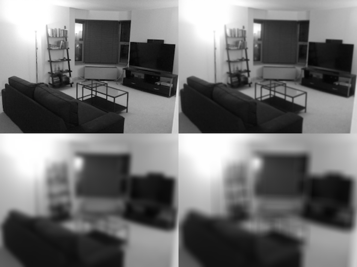
And, by allowing the user to control the sigma parameter, we can control how much
the kernel blurs. Below is the image convolved with \(\sigma\) = 0.01, 1.0,
5.0, and 10.0.
That’s basically it, but there are some little tweaks we could add. First, notice
how the Gaussian naturally tapers out; we can exploit this to functionalize the
kernel size based on the inputted sigma value. This can be done analytically (ie.
if you want the cutoff to be no more than 0.5%, then your kernel size needs to be
greater than \(1+2\sqrt{-2 \sigma^2 \ln{0.005}}\)).
The cutoff equation above was derived by defining the percentage threshold \(p\) as:
\(p = \frac{g(0,r)}{g(0,0)} = \frac{\frac{1}{2\pi\sigma^2}e^{-\frac{r^2}{2\sigma^2}}}{\frac{1}{2\pi\sigma^2}e^{0}}\)
This simplifies to \(r=\sqrt{-2\sigma^2\ln{p}}\). The rest of the equation is
a nomenclature change, with the minimum diameter \(d=1+2r\).
With that kind of logic, large sigma values make bigger kernels, which result
in more blurring. Here is \(\sigma = 10\) again, but with a generated kernel
size of 69.
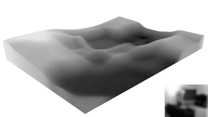
To be honest, I just wanted to run the picture through my 3D-izer. You have to admit that looks cool.
Additionally, the Gaussian function is symmetric, so you can separate the 2D convolution into two 1D convolutions. This provides a speed boost, although I honestly don’t think that speed is an issue here.
In the next section, we will go through using convolution and Fourier transforms to find underlying patterns in images.