Fourier transforms are something that come up all the time in science, so they’re worth including here. That being said, they’re a lot more specialized than taking gradients or blurring an image, so I won’t be offended if you gloss over this part.
At their core, Fourier transforms are really simple. Taking the one-dimensional example of audio signal processing, let’s say you have some music that produces noise like this:

This pattern is a sum of sinusoidal waves, each representing the frequency of some sound. You’ll notice, however, that we don’t know any of the frequencies.
In a Fourier transform, we aim to find this information out by brute force. Simply,
we multiply the above data by \(\sin{\omega x}\), where we keep varying \(\omega\).
If our guess for \(\omega\) does not coincide with a frequency, then the resulting
output is more noise. However, if it does fit, the output function is always positive,
as there is now a \(\sin^2{\omega x}\) term kicking around.
Because I wrote this function and this is all hypothetical, I can show you what’s going on mathematically. The above noise is the sum of three sine waves,
\(f(x) = \sin{1.2x}+\sin{2.5x}+\sin{6.0x}\)
Now, I’m going to multiply by some random \(\omega\) values. If \(\omega\)
is 0.5, you get random stuff.
\(\sin{0.5x}*f(x) = \sin{0.5x}\sin{1.2x}+\sin{0.5x}\sin{2.5x}+\sin{0.5x}\sin{6.0x}\)

The result is sometimes positive, and sometimes negative. If you sampled a bunch of values and added them up (ie. get the area under the curve), they’d probably wash out to approximately zero.
But, if \(\omega\) is 1.2, you get a squared sine term.
\(\sin{1.2x}*f(x) = \sin^2{1.2x}+\sin{1.2x}\sin{2.5x}+\sin{1.2x}\sin{6.0x}\)

A sine wave can have positive or negative values, but any real number squared is always positive. This makes the sine wave more positive overall. So, if you added together a bunch of samples, you’d have a large positive value.
If you guess the right frequency, you have a large value. Otherwise, you have nothing. That’s it!
Let’s apply this to images. Unlike the above example, images are two dimensions.
So, our sine wave has two arguments - frequency and direction. Through some basic
trigonometry, our \(\sin{\omega x}\) becomes \(\sin{\omega r}\), where
\(r = \cos{\theta x} + \sin{\theta y}\). Now, we need to multiply the image
by sine waves and add up the values. Which, if you think about it, is exactly
what we were doing with convolution.
So, we can generate a sinusoidal kernel:
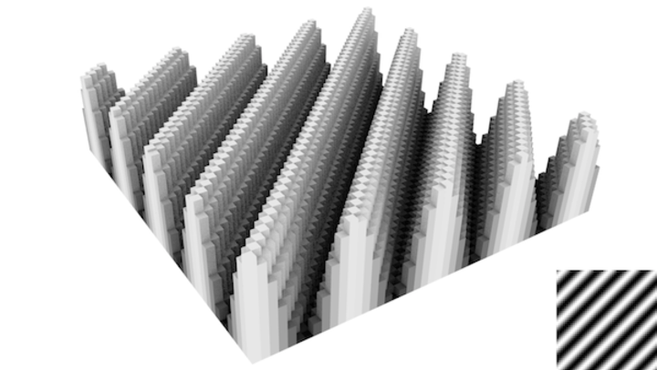
and convolve the kernel with an image.
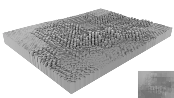
This doesn’t look like much, but there is information here. The peaks in the data
correspond to areas where the kernel found a pattern. In this case, my IKEA table
was placed at an aesthetically pleasing 45-degree angle. which coincided with the
Fourier \(\theta\).
Now, there are some issues here. In a true Fourier transform, the kernel would
have to cover the entire image on each iteration. The data would be more conveniently
plotted as a graph of \(\theta\) vs. \(\omega\). A picture of my living room
is a terrible example of an image that would have an interesting Fourier transform.
But, I’m not going to harp on these. Why? Because, in most cases, you won’t want
to directly use a Fourier transform on images. You’ll want to use the Gabor filter,
which I will introduce in the next section.
But, before that, math: the Fourier transform equation.
\(F(\omega,\theta) = \mathcal{F}[f(x,y)] = \frac{1}{\sqrt{2 \pi}}\iint f(x,y) e^{i \omega (\cos{\theta x} + \sin{\theta y})}\,dy\,dx\)
This is slightly different from the version you’ll usually see, as I wrote out
two dimensions of data. It looks complicated, but remember that \(e^{i\omega r}\)
is, by Euler’s formula, \(\cos{\omega r} + i\sin{\omega r}\). Add in the fact
that I have no idea how imaginary numbers would ever play a role in image
processing, and the equation simplifies to what we were doing. Guess a frequency
(and, in 2D, direction), multiply by a sine wave, integrate to see if it’s positive.
In the next section, we will combine the Fourier transform and the Gaussian blur to make something truly useful.