In the last two sections of this tutorial, we discussed Gaussian blur and Fourier kernels. The Gaussian kernel is good at weighting neighbors by their proximity to the pixel of interest, and the Fourier kernel gives us information about patterns in the image. So, uh, let’s… multiply… them?
\(gabor(\sigma, \omega, \theta) = gaussian(\sigma) * fourier(\omega, \theta)\)
Look at that. New filter. When kernel-ized, it looks like:
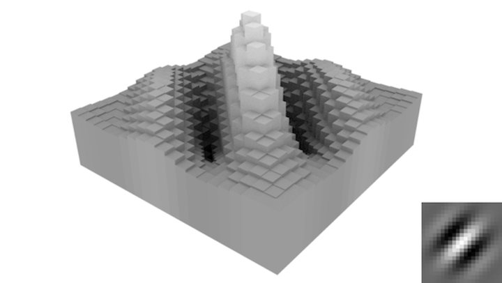
Its functionality can be summarized by taking the descriptions of the Gaussian and Fourier kernels and mashing them together. Something like “finding local patterns”. As most images don’t have universal patterns (like, say, a sound wave does), this is a very useful kernel. Also, every single paper that ever uses the Gabor kernel cites it as the best approximation of how humans process visual data. Seeing how I don’t even know how to explain color to a blind man, I have no idea how someone verified this claim. But, whatever. It’s cool, right?
Algorithms involving the Gabor kernel most frequently pop up in scenarios where one needs to test images for similarity; namely, they’re at the core of reverse image searching and fingerprint detection. In my own work, I’ve managed to use them to reconstitute experimental image sequences that got jumbled together by lazy file naming schemes. Less exciting than fingerprint detection, but it did save us from having to redo a lot of annoying lab work.
There is one obnoxious issue with the raw Gabor filter: it has a lot of parameters!
It adopts the arguments from both the Gaussian and Fourier kernels, so image
characterization by raw Gabor can be rather time intensive. To circumvent this,
you commonly see some heuristics applied. In the
Gaussian
section, I talked about using the natural decay of the function to convert kernel
size into a dependent parameter. Additionally, we can relate the Gaussian decay
to the wavelength of the Fourier function, removing the \(\sigma\) parameter
entirely. Coding this all up:
/**
 * Convolves image with a Gabor kernel
 */
float[][] gabor(float[][] img, float wavelength, float direction) {

  // Overwriting sigma with octaval value (the standard is to use one octave)
  float octave = 1;
  float sigma = wavelength * 1/PI * sqrt(log(2)/2) * (pow(2,octave)+1)/(pow(2,octave)-1);

  // Getting the required kernel size from the sigma
  // threshold = 0.005, x is minimum odd integer required
  int x = ceil(sqrt(-2 * sigma * sigma * log(0.005)));
  if(x % 2 == 1) x++;

  // Generate a kernel by sampling the Gaussian and Fourier functions
  float[][] kernel = new float[2*x+1][2*x+1];
  int uc, vc;
  float f, g, theta;
  for(int u=0; u<kernel.length; u++) {
    for(int v=0; v<kernel[0].length; v++) {
      // Center the Gaussian sample so max is at u,v = 10,10
      uc = u - (kernel.length-1)/2;
      vc = v - (kernel[0].length-1)/2;

      // Calculate the Gaussian
      g = exp(-(uc*uc+vc*vc)/(2*sigma*sigma));
      // Calculate the real portion of the Fourier transform
      theta = uc * cos(direction) + vc * sin(direction);
      f = cos(2*PI*theta/wavelength);
      kernel[u][v] = f*g;
    }
  }
  // Convolve and return
  return convolve(img, kernel);
}
While there is much more to learn in the field of image processing, I’m choosing to end my tutorial here. Why? Primarily, I have found that convolution is the most conceptually complex part of image processing. Once this concept “clicks” with a new student, much of the remaining techniques in the field fall into place with little effort. I hope that by focusing on this sub-topic, I have helped soften the image-processing learning curve and have enabled cool new scientific projects.
If you’re looking to continue increasing your knowledge in image processing, I recommend going straight to the literature. I know this sounds crazy - you’ve only started in the field - but, if you keep in mind the mathematical simplifications I discussed throughout the tutorial, papers in this field read very easily.
A great place to start would be Canny edge detection, which detects edges in an image by applying a Gaussian blur, then a Sobel gradient, and then some fancy terms (non-maximum suppression and recursive hysteresis) that encode very basic operations (make edges one pixel wide by keeping the strongest gradients, and have threshold values to control what is considered an “edge”). You could build this starting from the gradient lesson (which, on its own, is a decent edge detector), then add in noise-reduction pre-processing with a blurring operation, and then tackle the complex sounding stuff, if needed.
Another one is combining the Gabor filter with Earth Mover’s Distance metrics to create a reverse-image-search program. This is not nearly as difficult as it sounds. The earth mover’s distance is easy to visualize as a tractor moving piles of dirt into holes (therefore, the name), and the Gabor filter shown above is nothing more than a tool to emphasize localized textures in an image.
Finally, you can easily use these tools to make your (or your friends’) experimental work easier! For example, let’s say you are tracking a cell with a microscope that has a computer interface. The cell keeps moving, so someone is forced to sit in the lab for hours on end moving the lens to keep the cell approximately centered. That’s annoying and repetitive. Fix that. In this case, you can use a threshold filter (or edge/blob detection, if you’re feeling fancy) to find the cell in each recorded tracked frame. Find the centroid by averaging all of the pixels constituting the cell, and then find a way to get the script to move the microscope to recenter the cell (good microscopy software offers an API and documentation to do this; with bad software, you could run a mouse-clicking macro to achieve the same effect).
Once again, I hope these lessons helped. If you’ve been doing anything interesting with image processing in the lab, leave a comment below!